5.1.4.3. Considerations of the velocity profile
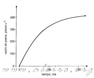
The velocity profile can be built if this expression is evaluated, for example for some values of f:
| f (steps * s -1) | t (ms) |
| 100 | 21 |
| 150 | 32 |
| 200 | 46 |
| 250 | 61 |
| 300 | 84 |
| 350 | 117 |
| 400 | 177 |

Figure 5.9. Optimum velocity profile resulting from evaluating the equation 5.24.
The full velocity profile shown in Figure 5.9. Since this result is derived from the characteristic approach to pull-out torque which is a couple less than the actual curve, the engine must be able to follow the profile of a uniform rate if the load remains within the expected. In the first installment of 0-100 steps * s -1 the profile has a linear form, this is because the engine torque characteristic T (f) and the load T L (f) are constant, the following we have an exponential acceleration section with a more pronounced in the low ratio of steps taken advantage of the available engine torque for these reasons of steps to speed as quickly as possible, the higher the rate of steps the slope levels gradually reach the pull-out ratio to a zero acceleration. Because with increasing engine speed, it loses torque and therefore the ability to accelerate. The torque motor delivers distributed drag friction load T (f) and particularly in accelerating the inertia of the system, reaching the final with a zero acceleration, delivering all the torque you have to drag friction load.
When the system is decelerating, the engine must produce a negative torque and therefore each phase must be activated after the rotor passes the equilibrium position of the phase. The load angle defined in paragraph 3.2.2 is then negative and the motor produces a braking torque T B (f), which is usually larger than the pair of pull-out [T B (f)> T ( f)]. The equation of motion of the system is then:
\ =\ T_L(f)+J*\left( \frac{\partial^2 \theta }{\partial t^2} \right)) (5.25)
(5.25)
Where T B (f) is the pair of deceleration to the ratio of step f. Substituting for df / dt in terms of f of Equation 5.16 yields:
![df / dt in terms of f \frac{\partial f}{\partial t}\ = \ -[T_B(f)+T_L(f)]*\frac{n*p}{2*\pi *J}](http://www.alciro.org/cgi/tex.cgi?\frac{\partial f}{\partial t}\ = \ -[T_B(f)+T_L(f)]*\frac{n*p}{2*\pi *J}) (5.26)
(5.26)
When the load torque due to inertia of the system helps the engine torque, the optimal speed profile during deceleration can be obtained by integrating the above equation:
-T_L(f)}) (5.27)
(5.27)
where t is the time to decelerate from the reason why steps f f i initial steps. To integrate the function 1 / [T B (f) + T L (f)] should be used again the graphic method. A typical optimal speed profile of this integral as shown in Figure 5.6.


